4 Sail design
4.1 Restrictions on the Sail Design
The sail design is primarily restricted by the International Moth class rules. These rules are written in full in Appendix 1. The relevant rules are summarised below.
·
There may be only one sail on the boat when racing.· The measured and calculated area, using the IYRU method of sail area calculation, shall not exceed 8m2.
· Only the area of that part of the spars that will not pass through a ring of 90 mm internal diameter shall be included in the area calculation.
· For a sail which encloses the mast an area equivalent to the length of the luff multiplied by 50 mm shall be excluded.
· For a sail which encloses the boom an area equivalent to the length of the foot multiplied by 90 mm shall be excluded.
·
No attempt at increasing sail area shall be made by the number or size of battens used.·
The luff length of the sail shall not exceed 5.185m.
The operating conditions of the sail can be split into two distinct categories which correspond to an under and overpowered state. The mast and sail should be designed within the rules to provide a minimum drag and maximum drive when under powered. However, once the maximum heeling moment produced by the sailor's weight has been reached, the mast and sail must be de-powered by reducing lift and drag. This posses another restriction on the sail design.
The most obvious way to reduce lift and drag is to decrease the sail area. However, although this may be possible on the shore by reefing or changing sails, it will be too difficult and time consuming during a race. More sophisticated methods of de-powering the sail must be investigated as part of a complete design.
4.2 Basic Sail Performance Characteristics
Figure 4.1 shows the lift and drag characteristics of a single sail. If a hull is superimposed onto this diagram, with an apparent wind angle to the boat b and to the sail a , the best sail setting position can be identified.
A corresponds to a minimum aerodynamic drag angle.
B corresponds to a maximum forward drive force.
Altering the sheeting angle to move along the polar curve from A to B causes an increase in side force as well as an increasing drive force. Extra dagger board induced drag is created as side force increases. Initially sail drive exceeds the increase in drag and boat speed increases. Ultimately the reverse occurs and there is a point of optimum boat speed somewhere between A and B.
In moderate weather where the craft is under powered this optimum is the proper choice of sail setting. Sailing close hauled, the optimum is nearer A than B. In reaching conditions it is nearer B, and B itself approaches the point of maximum sail lift coefficient.
In heavy weather it is necessary to reduce sail power in order to reduce heeling moments. The apparent wind angle must be decreased by sheeting out and/or pinching (decreasing b ). This has a dramatic but limited effect on the heeling moment. The sail becomes less powerful but has more drag as a decreases past A.
The lift and drag polar curve must be optimised for each wind strength and point of sailing, if the best performance of the sail is to be realised.
4.3 Spanwise Lift Distribution
"Towards an Optimum Yacht Sail"
Wood and Tan
Journal of Fluid Mechanics 1978
"Sail Optimisation for High Speed Craft"
A H Day
RINA 1990
"The Optimisation of Aerodynamic Lift Distribution for a Heeled Yacht in a Wind
Gradient"
A H Day
RINA 1991
The above papers, which investigate optimum spanwise lift distribution, raise the following points.
·
The effect of the gap below a sail has a significant effect on both the optimal sail plan and the attainable performance (figure 4.2).·
The wind gradient has little effect on optimal spanwise lift distribution.·
Where sail area is limited to a maximum value, and the boat is under powered, an elliptical sail plan is optimum.·
In an overpowered state the lift produced by the head of the sail must be reduced to decrease the heeling moment.·
If the practical problems can be overcome, reverse circulation at the head of the sail produces and increase in performance (for the same heeling moment) for high speed craft such as sail boards.
A Moth is too slow to be compared to a sail board and is not sailed heeled to leeward upwind like a yacht. Hence the graphs of optimum spanwise lift distribution ( figure 4.3 ) are not directly applicable. However, the above points can be incorporated into the sail design.
There is a large gap under a Moth sail so that the sailor can get across the boat. This means that there will be no lift generated at the boom as well as at the head of the sail.
The approximate lift distributions shown in figure 4.4, are suitable for an elliptical Moth sail in an under and an over powered state.
"C" and "D" indicate the approximate height of the centre of pressure for the two cases. "C" corresponds to the untwisted elliptical plan form. "D" corresponds to the same plan form but with a twisted leach to reduce the angle of attack and hence lift at the top of the sail. "D" is lower than "C" indicating that there will be less heeling moment for the same total lift.
In practice the heeling moment will remain constant and the sail will be twisted or untwisted depending on wind strength. This is clearly an effective and efficient method of de-powering a sail.
4.4 Sail Section Design
The section of the sail will have a large effect on its characteristics. Figures 4.5, 4.6 and 4.7 show the dramatic effects that the section shape has on the lift and drag generated by a single sail.
A suitable sail section must be chosen to give good performance on all points of sailing and in most wind strengths. The section of the sail is under the control of the sail maker who will shape the sail on the basis of years of empirical experience. Without extensive wind tunnel tests the sail maker's intuition must be trusted.
The way the sail is attached to the mast has a very dramatic effect on the flow over the sail and hence pressure distribution as shown in figure 4.8.
It is possible to sleeve the sail over the mast. Camber inducers on the ends of the battens inside this sleeve create a far better shape than the normal circular mast and bolt rope assembly (figure 4.9).
The methods of sleveving the sail onto the mast, to simulate a wing mast and sail configuration, has been developed by wind surfer sail manufacturers. It has several advantages over wing masts and conventional masts which are as follows.
·
There is no need for a track to be fitted to the mast which saves significant weight. (The author has found that form his experiments with camber induced sails, that a tubular carbon mast was 1 kg lighter than a 3.5 kg conventional carbon mast with a moulded sail track.)·
The mast section is a tapered circular tube which lends itself well to FRP fabrication.·
The modules, and hence bend characteristics, of the mast can be controlled well with uni-directional fibres if it is made from FRP. Due to its shape a wing-mast will not bend significantly fore and aft which could be a problem.·
The lift and drag characteristics of the rig are greatly improved by eliminating the separation bubble on the leeward side of the sail.·
When the sail is twisted the cloth sleeve will also twist, maintaining the correct shape all the way up the mast.
This type of sail is harder to rig than a conventional sail but it can be zipped on to the mast quite easily.
Much time and effort must be employed by the sail maker to achieve the correct camber induced shape, so that the full potential of the sail can be realised.
The extra weight and expense of a sail with camber inducers is easily justified by the cheaper lighter mast and potentially superior lift and drag characteristics.
4.5 Sail Plan and Area Measurement
The sail profile design has an elliptical cord distribution along its span as
shown in figure 4.10. The measurement points and formulae used to calculate the area of
the sail (in accordance with the rule in Appendix 1) are also shown.
The luff tube has not been shown but it would be sewn on with its front edge 50 mm in front of the drawn luff curve. This would therefore not be included in the measurement of the area of the sail under rule 9.2.(iii) ( ref. Appendix I ).
Sail Area Measurement
AB = 5.1
BC = 1.7
AC = 5.05
d = 0.78
e = 0.80
f = 0.6
g = 0.2
h = 0.025
S = (AB + BC + AC)/2 = 5.925
Area of main triangle = Ö
S(S-AB)(S-BC)(S-AC)
= 4.251
Area of luff round = 2/3 AY.g
= 0.68
Area of foot round = 2/3 XC.h
= 0.028
Area of leech round = AC/4 (1.16d + e + 1.16f)
= 3.031
Total area = 7.99 m2
(Note: Total area < 8m2 rule 9.2 )
4.6 Foil Angle of Sweep
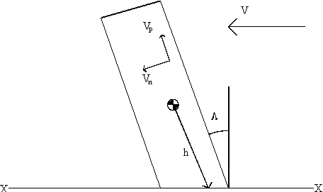
The optimum angle of sweep is a complicated problem to solve, especially as there is not much published data to analyse. However, figure 4.11 shows how induced drag varies with angle of sweep and the following crude mathematical analysis helps us to understand how lift and drag are affected by angle of sweep.
V = free stream velocity
VN = component of V normal to the mid cord line
VP = component of V parallel to the mid cord line
h = distance along foil from its root to the centre of pressure
L = lift
CL = lift coefficient for foil
CDP = profile drag coefficient for foil
CM = moment coefficient for foil about X-X of lift
L = angle of sweep of the 1/4 cord line
CDPN = drag coefficient component normal to mid cord
CDPP = drag coefficient component parallel to mid cord
VN = V cos L
VP = V sin L
CL µ VN2
CL µ cos2 L
Assuming Vp does not contribute to the lift produced by the foil.
CM µ L h cos L
CM µ cos3 L
Assuming that h is constant in that the centre of pressure does not move.
CDPN µ VN2
CDPP µ VP2
The addition of both components in the direction of the free stream will give the total profile drag coefficient CDP
CDP µ VN2
cos L + Vp2 sin L
CDP µ cos3 L + sin3 L
Therefore we have
CL (swept) / CL (unswept) = cos2 L
CM (swept) / Cm (unswept) = cos3 L
CDP (swept) / CDP (unswept) = cos3 L + sin3 L
CDI (swept) / CDI (unswept) = taken from figure 4.11
Table 4.1
Calculated values of CL and CD for a foil with sweep where induced and profile drag are equal in magnitude.
| L | CL | CM | CDP | CDI | CD | CL/CD |
| -4 | 0.995 | 0.993 | 0.993 | 1.022 | 1.0075 | 0.988 |
| -2 | 0.999 | 0.998 | 0.998 | 1.015 | 1.0065 | 0.993 |
| 0 | 1 | 1 | 1 | 1.009 | 1.0045 | 0.996 |
| 2 | 0.999 | 0.998 | 0.998 | 1.004 | 1.001 | 0.998 |
| 4 | 0.995 | 0.993 | 0.993 | 1.001 | 0.997 | 0.997 |
| 6 | 0.989 | 0.984 | 0.985 | 1.001 | 0.993 | 0.996 |
| 8 | 0.981 | 0.971 | 0.974 | 1.004 | 0.989 | 0.992 |
| 10 | 0.970 | 0.955 | 0.960 | 1.009 | 0.9845 | 0.985 |
| 12 | 0.957 | 0.936 | 0.945 | 1.015 | 0.980 | 0.977 |
| 14 | 0.941 | 0.914 | 0.928 | 1.022 | 0.975 | 0.965 |
| 16 | 0.924 | 0.888 | 0.909 | 1.031 | 0.970 | 0.953 |
| 18 | 0.905 | 0.860 | 0.890 | 1.042 | 0.966 | 0.937 |
| 20 | 0.883 | 0.830 | 0.870 | 1.055 | 0.9625 | 0.917 |
| 22 | 0.860 | 0.797 | 0.850 | 1.069 | 0.9595 | 0.896 |
| 24 | 0.835 | 0.762 | 0.830 | 1.084 | 0.957 | 0.873 |
| 26 | 0.808 | 0.726 | 0.810 | 1.100 | 0.955 | 0.846 |
| 28 | 0.780 | 0.688 | 0.792 | 1.120 | 0.956 | 0.816 |
| 30 | 0.750 | 0.650 | 0.775 | 1.135 | 0.955 | 0.785 |
Table 4.1 and graph in figure 4.12 use the assumption that profile drag and induced drag are the same in magnitude and so CD is their average. However, from figure 4.13 it can be seen that this may not necessarily be the case. I shall re-analyse the data using a revised assumption that induced drag is 50% greater than the profile drag.
\ CD = (1.5 CDI + CDP) / 2.5
Table 4.2
Calculated values of CL and CD for a foil with
sweep where induced is 50% larger than profile drag.
| L | CL | CDP | CDI | CD | CL/CD |
| -4 | 0.995 | 0.993 | 1.022 | 1.010 | 0.985 |
| -2 | 0.999 | 0.998 | 1.015 | 1.008 | 0.991 |
| 0 | 1 | 1 | 1.009 | 1.005 | 0.995 |
| 2 | 0.999 | 0.998 | 1.004 | 1.002 | 0.997 |
| 4 | 0.995 | 0.993 | 1.001 | 0.998 | 0.997 |
| 6 | 0.989 | 0.985 | 1.001 | 0.995 | 0.994 |
| 8 | 0.981 | 0.975 | 1.004 | 0.992 | 0.989 |
| 10 | 0.970 | 0.960 | 1.009 | 0.989 | 0.980 |
| 12 | 0.957 | 0.945 | 1.015 | 0.987 | 0.970 |
| 14 | 0.941 | 0.928 | 1.022 | 0.984 | 0.956 |
| 16 | 0.924 | 0.909 | 1.031 | 0.982 | 0.941 |
| 18 | 0.905 | 0.890 | 1.042 | 0.981 | 0.922 |
| 20 | 0.883 | 0.870 | 1.055 | 0.981 | 0.900 |
| 22 | 0.860 | 0.850 | 1.069 | 0.981 | 0.876 |
| 24 | 0.835 | 0.830 | 1.084 | 0.982 | 0.850 |
| 26 | 0.808 | 0.810 | 1.100 | 0.984 | 0.820 |
| 28 | 0.780 | 0.792 | 1.120 | 0.989 | 0.789 |
| 30 | 0.750 | 0.775 | 1.135 | 0.991 | 0.757 |
Graph 4.2 shows that the optimum angle of sweep of the 1/4 cord line of the main sail is 3° . However, the following assumptions must be born in mind.
·
Induced drag is 50% larger than profile drag.
· The graph in figure 4.11 and 4.13 can be applied accurately to a Moth main sail.
· The crude mathematical analysis is accurate enough to represent the characteristics of the Moth sail.
Moth sailors tend to sail around with a mast rake of around 5° which indicates a 1/4 cord line angle of sweep of 3° . (Note: the difference between mast rake and maximum depth rake angle is measured from figure 4.10.). This value has been derived empirically so its validity is questionable but it does agree with the mathematical derivation of the optimum angle of sweep which helps validate both approaches.
The boat should be rigged with 5° of mast rake to be optimum for under powered conditions up wind. This will define a set of conditions for which the centre of lateral resistance and centre of effort of the sail can be balanced.
In over powered conditions the mast can be raked to decreases the heeling moment of the sail. This decreases the efficiency of he sail but a raked full sail is more efficient than an upright stalled sail.
If the 1/4 cord line of the sail is raked by 15° to 18° the heeling moment will be reduced by 14%. There is no real practical limit to mast rake, only a control problem. If the boat is balanced with 5° of mast rake it will be unbalanced with 20° of rake. A degree of unbalance is not a problem but more will eventually result in loss of control.
4.7 Mast Raking Systems
The details of an advanced mast raking system, used on an existing boat, are given in Appendix 2. The system relies on the fact that the shrouds and forestay are tied together and the join is moved on one control line. The position of the shroud and forestay mountings on the boat is critical so that rig tension is kept constant as the mast is raked.
Schematic diagram representing the mast and stay vectors
fx = Ox + Mx fy = Oy + My
fx = Ox + M sin a fy = Oy + M cos a
ç
f ç = Ö ( fx2 + fy2 )Sx = Nx + Mx Sy = Ny + My
Sx = Nx + M sin a Sy = Ny + M sin a
SZ = NZ
ç
S ç = Ö ( Sx2+ Sy2 +SZ2 )For a given shroud position and hound height, ç M ç an N are known. For different mast rake angles a 1 and a 2, ç S1 ç and ç S2 ç can be calculated. O is the vector to a fixed line corresponding to the centre line of the foredeck. So for various forestay positions along this line ç F1 ç and ç F2 ç can be calculated. If P is the ratio of forestay to shroud purchase. The above calculation can be done in an iterative manner to find the correct forestay position where P is some integer value that can be achieved with a simple block and tackle system.
P = ( ç F1 ç - ç F1 ç ) / ( ç S1 ç - ç S2 ç ) » 3
This process would lend itself well to an iterative computer programme written to find O for a given P, N and M.
4.8 Sail Controls and Their Effects
We have seen how sail twist, camber, draft, position, etc have a large effect on the lift and drag curve and that this curve needs to be optimised for each point of sailing. Once the boat has been launched the only influence that can be achieved over the shape of the sail is by adjusting control lines. These have various effects; so to tune the boat effectively an understanding of how to achieve the optimum characteristics of the sail is necessary.
Figures 4.15, 4.16 and 4.17 show the effect of kicker tension. We must be wary of this experiment as it may be more an investigation of decreasing gap than decreasing twist ( Ref figure 4.2 ). Taking a simplistic view of the data we can assume that kicker tension increases upwind performance by moving point "A" (minimum aerodynamic drag angle) to the left on the polar curve. and easing the kicker to a certain degree increases the value of "B" (maximum lift) which is beneficial on a reach. This may be explained by following points.
·
Kicker tension reduces twist and increases mast bent.·
Reducing twist increases the angle of attack of the sail at its head. This would increase upwind performance when under powered.·
Mast bend removes shape from the front 1/3 of the sail which is detrimental to upwind performance.·
Increasing kicker tension reduces the gap under the boom which increases performance.·
CL maximum is a function of camber so kicker tension flattens sails with mast bend and decreases CL maximum.
The above effects all play a part in adjusting the sail characteristics. As they all interact it is hard to isolate and quantify each effect.
Figure 4.18 shows the effect of foot and luff tension on a Fin sail.
Run VI is the control run.
Run X was done with the foot stretched.
Run XII was done with both the foot and luff tensioned.
The graph shows that these control lines can have a significant effect and must be tensioned correctly when racing.
The data in figures 4.15, 4.16, 4.17 and 4.18 can not be directly applied to a Moth sail because it is very different from a Finn's sail, but they do help us to understand how to tune the boat.